
Learning Objectives
Following this assignment students should be able to:
- integrate programing fundamentals and working with data
- solve a data analysis problem with logical and automated code chunks
- communicate effectively with informative and well-styled R scripts
Reading
-
Topics
- Style
- Debugging
-
Readings
Lecture Notes
Exercises
-- Size-biased Extinction --
There were a relatively large number of extinctions of mammalian species roughly 10,000 years ago. To help understand why these extinctions happened scientists are interested in understanding whether there were differences in the body size of those species that went extinct and those that did not.
To address this question we can use the largest dataset on mammalian body size in the world, which has data on the mass of recently extinct mammals as well as extant mammals (i.e., those that are still alive today). Take a look at the metadata to understand the structure of the data. One key thing to remember is that species can occur on more than one continent, and if they do then they will occur more than once in this dataset. Also let’s ignore species that went extinct in the very recent past (designated by the word
"historical"in thestatuscolumn).Import the data into R. If you’ve looked at a lot of data you’ll realize that this dataset is tab delimited. Use the argument
sep = "\t"inread.csv()to properly format the data. There is no header row, so usehead = FALSE. The unknown value used in the dataset is-999. R assumes your unknown value isNA, but"NA"in the data is the code for North America. Use the additional argumentsstringsAsFactors = FALSE, na.strings = "-999"inread.csv()to get R to keep"NA"as a string and transform-999toNA.It’s probably a good idea to add column names to help identify columns:
colnames(mammal_sizes) <- c("continent", "status", "order", "family", "genus", "species", "log_mass", "combined_mass", "reference")- Create a new RStudio project and a new version control repository for this
exercise and commit your changes in small logical chunks. Make sure to commit
all of the files that are needed for the analysis to the repository. If you would like a private repository on GitHub please ask your instructor to set
one up. Throughout the assignment focus on using good style to make the code easy for you or someone else to read. - Calculate the mean mass of the extinct species and the mean mass of the extant species. Don’t worry about species that occur more than once. We’ll consider the values on different continents to represent independent data points.
- It looks like the species that went extinct are larger on average, but there
are lots of different processes that could cause size-biased extinctions so
it’s not as informative as we might like. However, if we see the exact same
pattern on each of the different continents that might really tell us
something. Repeat the analysis but this time compare the mean masses within
each of the different continents (
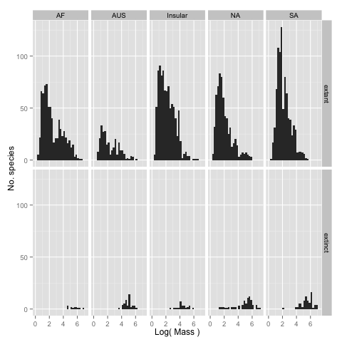
dplyrwould be one way to do this). Export your results to acsvfile where the first entry on each line is the continent, the second entry is the average mass of the extant species on that continent, and the third entry is the average mass of the extinct species on that continent (spread()fromtidyris a handy way to convert the standarddplyroutput to this form). Call the filecontinent_mass_differences.csv. - Looking at the averages was a good start, but we really need to look at the
full distributions of masses of the two groups to get the best picture of
whether or not there was a major size bias in extinctions during the late
Pleistocene. Make a graph that shows the data for each continent that you
think is worth visualizing. For each continent display two histograms (these
can be on the same axes or separate sets of axes) that use the same bins to
display the number of extinct and extant species. Use the
log_massrather than the mass itself so that you can see the form of the distributions more clearly.facet_gridorfacet_wrapmay be useful to laying out the subplots. Label the plots to make it clear to someone viewing them what they are looking at. Save the graph or graphs as.pngfile(s) (this should happen automatically in the code).
- Create a new RStudio project and a new version control repository for this
exercise and commit your changes in small logical chunks. Make sure to commit